
12/01: Day 1 🎄


Welcome to Unwrapping TPUs!
We migrated our blog from Notion to Substack! For those of you looking to follow along with notifications feel free to subscribe below. We also launched our Substack chat for further discussions outside of Twitter if you readers so fancy!
In the coming posts, we hope to cover the following topics:
Functional definition (The math needed in today’s compute, performance bottlenecks)
TPU teardown (Block by block, systolic array mechanisms)
Putting the TPU together (Synthesizing the TPU as a unit)
Let’s get started!!
Very very briefly, what is Google’s Tensor Processing Unit (TPU?)
In 2013, Google had just developed their flagship speech recognition model using DNNs and came across a frightening discovery. On the back of Jeff Dean’s napkin math, they noticed that if all of Google’s users spent ~3 min/day using speech recognition on apps like Translate or Search, Google’s existing global data center footprint would be overloaded by almost 2-3x alone.
Google’s early large-scale DNN models like PHIL had been trained purely on CPUs, lacking efficiency (In the Plex). With the launch of AlexNet and the rise of parallel usage of GPUs for scientific compute, Google needed a huge jump in the ability to conduct inference at scale cheaply.
The TPU was Google’s first strike at inference, specifically designed to handle the mathematical operations needed to run complex ML models fast.
What’s the math needed you ask? We start with the matrix multiply operation or MatMul.
Why MatMuls?
A MatMul is a matrix multiplying another matrix to produce .. another matrix. This single operation is what allows any and all modern ML algorithms to take data, learn, and produce predictions or generate data. To motivate intuition towards why the MatMul is so fundamental, we consider a variety of ML architectures.
Linear Algebra Fundamentals in Popular ML Architectures (circa TPU v1)
DNNs or Deep Neural Networks have been the centerpiece of recent AI developments, ranging in usage from data centers to our mobile phones. Inspired by the brain, DNNs are made up of artificial neurons that compute the output of a set of products of weight parameters and data values, passed through a nonlinear function or activation.
Clusters of these artificial neurons process different portions of input and feed their output into subsequent layer of neurons. The intermediary layers between input and final output are referred to as hidden layers.
Looking at the TPU v1 Paper (Jouppi et al.), six DNN applications (2x MLP, 2x LSTM, and 2x CNN) represented 95% of Google’s inference in 2016. We outline each of these types of DNN applications below and the math needed. Note that each of these are examples of supervised learning, which require training.
MLP (Multi-Layer Perceptron):
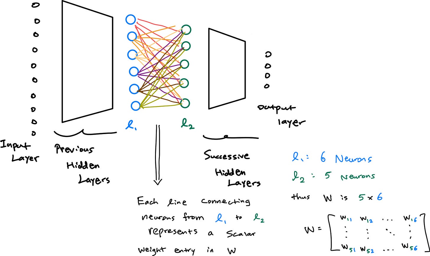
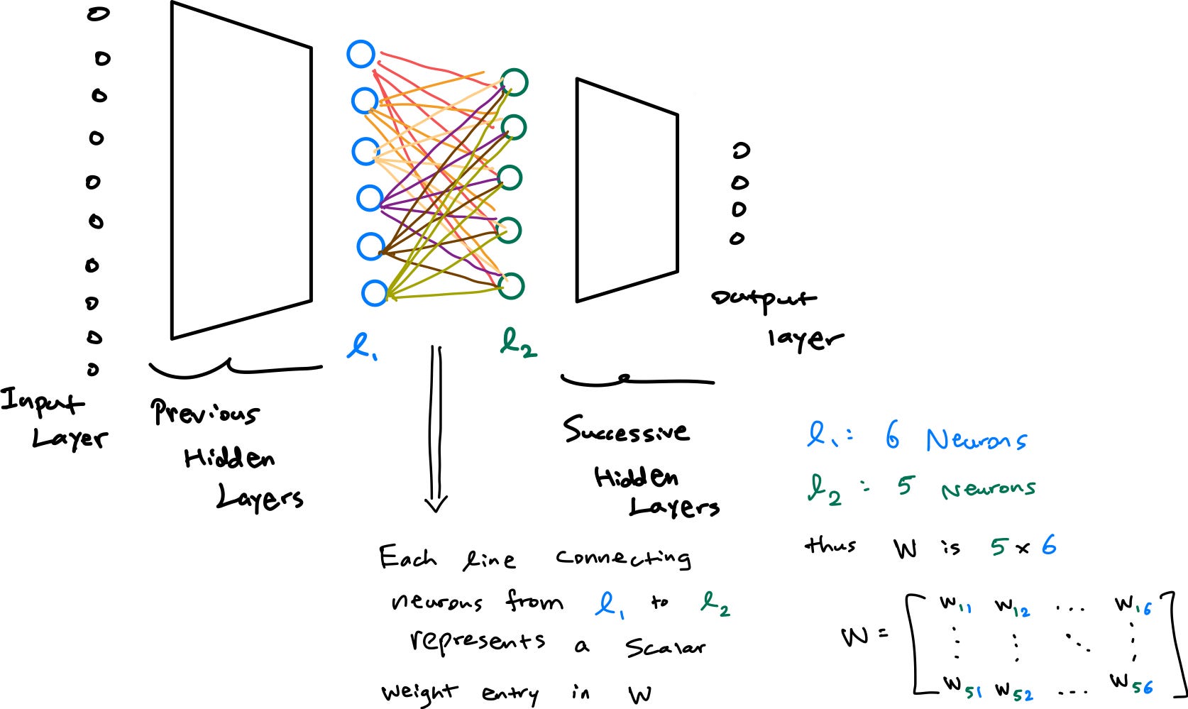
An MLP is a foundational architecture that connects an array of inputs to an array of outputs through a series of intermediate layers (hidden layers) where every single node (a neuron) in a given layer is fully connected to every single node in a subsequent layer
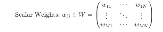
Let two subsequent layers in an MLP be denoted as l1 and l2, respectively. Each ‘connection’ of nodes between l1 and l2 are defined by scalar weights which collectively form a weight matrix that defines initial transformations for each neuron in l1 to l2. To put this more clearly, if l1 has N nodes and l2 has M nodes, the weight matrix W is an M x N matrix. Each entry w_ij in W is the scalar weight for connection of node j in l1 to node i in l2.
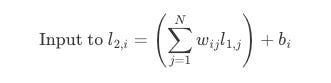
Now, the operation that defines the output of a single node in l2 is simply the dot product between the corresponding scalar value from W and the value of the node ! Let us consider node i in layer l2, its input value (before the activation function) is the sum of the products of every output l_1j from the previous layer l2 and its corresponding weight w_ij from the matrix W, plus a bias b_i:
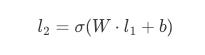
The matmul is now simply the computation of all of these individual dot products at once (it does the transformation above for all nodes in l2). In terms of an MLP, it introduces a non-linearity aspect per weight matrix through an activation function, sigma , which allows the model to learn relationships that are non-linear, aka the real world :) . The final output vector for layer l2 is:


As we can see, the matrix multiplication is the very operation that is allows an MLP and its neurons to ‘connect’ to each other and compute the weighted sum of inputs across each subsequent layer.
During training of an MLP, classical algorithms such as gradient descent simply adjust the entires of W (and the bias terms). Thus, training and forward pass of an MLP both boil down to iterative matrix multiplications between layers !
CNN (Convolutional Neural Network):
CNNs are a specialized type of DNN that applies nonlinear functions to local neighboring regions of the previous layer’s outputs. The dense amount of local connectivity and weight reuse allows CNNs to capture spatial patterns and reduce the number of parameters compared to fully connected layers.
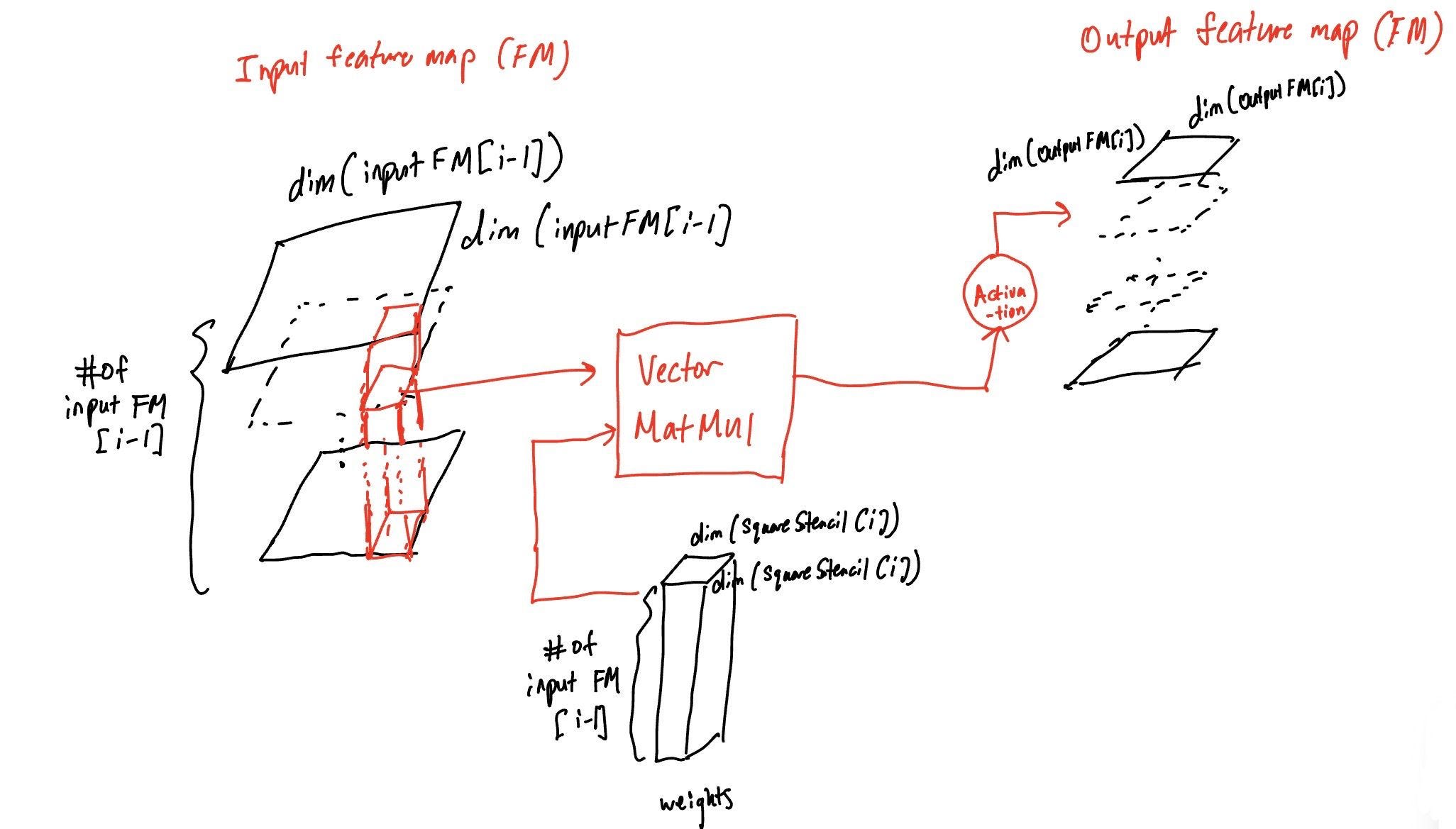
Each neuron layer produces a 2D feature map, where each cell of this feature map is tied to the identification of one feature in the corresponding input. This compression of parameters can be thought of how a CNN “learns” to classify.
In the following diagram (referenced from Hennessy and Patterson Fig 7.9), we see the feature map passage between input and output layers, augmented by a vector MatMul w/ weights. Due to the number of neurons and weights involved in these MatMul operations, CNNs can have less weights but greater arithmetic intensity than fully-connected MLPs.
RNN (Recurrent Neural Network):
Last but not least, RNNs focus on the ability to model sequential inputs with states (think of an FSM). Each layer of an RNN is a weighted sum of inputs from prior layers and previous states, forming what can be thought of as a memory.
The TPU v1 paper in particular focuses on LSTMs or Long Short-term Memory, where an LSTM has additional functionality keeping track of both a hidden state (output at each step or short-term memory) and the cell state (the long-term memory). At each time step, the LSTM decides what to forget (forget gate), what information to add (candidate cell state gate), and what to output (output gate). Each of these decisions can be thought of as gates, wherein each gate performers a Matrix-Vector multiplication.
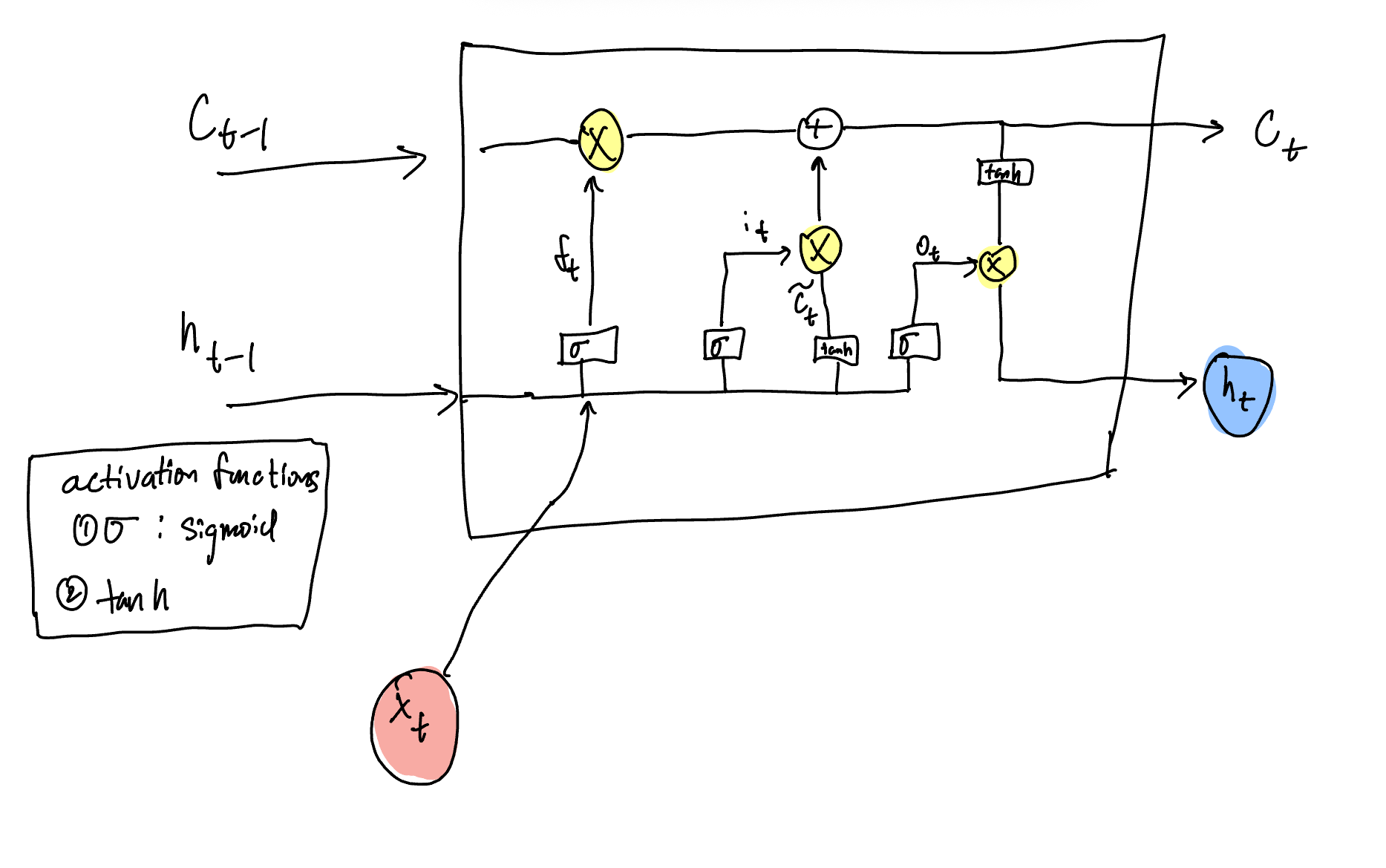
A great visual drawn from Sun et al. breaks down the exact MatVect operations at the junctions highlighted in X. From left to right inside of the LSTM block are forget gate, input gate, candidate cell state gate, and output gate.
Why hardware acceleration matters
ML models like MLPs, CNNs, RNNs, etc (don’t worry we will get to the etc soon) place high computational load on hardware. The core operations behind these models are dense matrix multiplies, repeated thousands to millions of times. CPUs aren’t built for workflows where the execution of massive numbers of identical arithmetic operations is necessary. We know GPUs offer thousands of lightweight cores that can chew through large streams of data at once. The GPU architecture allows for massive parallelism and high memory bandwidth, perfect for ML. TPUs take the optimization of the GPU a step forwards and offer for specific complex instructions (CISC) strong benefit given that the calls are regular and frequent.
Works Referenced / Further Reading:
Steven Levy, In The Plex: How Google Thinks, Works, and Shapes Our Lives.
Acquired Podcast, Google: The AI Company
John Hennessy and David Patterson, Computer Architecture 6th Edition (Chapter 7.1, 7.2)
Jouppi et al. In-Datacenter Performance Analysis of a Tensor Processing Unit
Sun, Qingnan & Jankovic, Marko & Bally, Lia & Mougiakakou, Stavroula. (2018). Predicting Blood Glucose with an LSTM and Bi-LSTM Based Deep Neural Network. 1-5. 10.1109/NEUREL.2018.8586990.
🐐🐏