12/15: Day 15 🎄

Inference! Land ho at last!!

Welcome back to Unwrapping TPUs ✨

We’ll keep it concise today as we wrap up our tiny^2 TPU setup. Yesterday, we got to a pretty exciting point, having previously established the feedback dataflow path and now the forward dataflow path to feed the MMU systolic array. Today, we demonstrate full inference for the very first time in the case of a forward pass on the 2-layer MLP.

(SVG w/ help from Opus 4.5)

2-Layer MLP Forward Pass

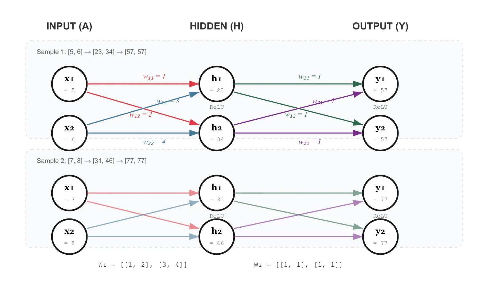
Our MLP integration sits in mlp_integration_tb.v in our Github, such that the network computes for an end result Y = ReLU(H x W2) after layer 2 of the MLP where H = ReLU(A x W1) for initial activations A and Weight stream W_1 for the first layer of the MLP (A - input activations, H - hidden representations, and Y - final output). Capitulating these two equations, the two layers folded in are Y = {y1, y2} = ReLU(ReLU(A x W1) x W2).

This architecture validates the TPU’s ability to chain MMU systolic array operations by feeding quantized outputs of one layer back into the Unified Buffer for the subsequent layer 2 calculations.

Layer 1: Input —> Hidden

Layer 1 receives the input activation matrix A of depth 2, in our example, which is instantiated as [[5,6], [7,8]] and multiplies A by weight matrix W1 = [[1,2], [3,4]]. The systolic array computes H as (A x W1) in the MMU initially before being applied with ReLU in the Activation Pipeline. Each PE of the MMU holds one weight element and activations stream through horizontally while partial sums accumulate vertically.

Observe the top left for PE00 (row, col). It starts with activation 5 and weight 1 which is added to subsequent PE10 which adds 6 * 3 making a resultant final Y1 output of 23. Similar operations hold for the right column. Since all values are positive, the ReLU activation function passes through unchanged. The activation pipeline then applies identity normalization and quantizes the 32-bit accumulator values into INT8 feeding back an end hidden layer of [23, 34] for the initial pair of activation inputs and [31, 46] for the two second wave of activations. In our diagram above, we split these up into a top and bottom channel just for ease of viewing, in reality these values are combined in computation.

Layer 1 to Layer 2: Data Transfer

Between layers, we drain layer 1’s results through the activation pipeline and enter a transfer FSM state where quantized outputs are refilled for the next layer’s results. Each activation pipeline pulse or ap_valid bit delivers one complete result row {y1, y2} where each of the columns are outputted together.

We then refill the unified buffer in reverse order as the hidden layer calculations are pushed through for one final layer 2 calculation round as {34, 23} and {46, 31} for the two deep wave of calculations. Implicitly, we cycle out the initial unified buffer we call A to receive outputs and into a unified buffer B to ferry in the next round of calculations with buffer A moving into position to collect for the Y outputs. The weight FIFO is reset to load in W2, which is [[1,1], [1,1]].

Layer 2: Hidden —> Output

Receiving H from UB “B”, we multiply by W2. Since W2 is all ones, each output element is easily verified as the sum of the corresponding input row such that for output rows, we have Y = {57 = 23 + 34, 57} and {31 + 46 = 77, 77} for rows 0 and 1 respectively. The ReLU once again passes through smoothly for positive values, producing the final output Y as we’ve just described.

 2 layer MLP test

 Network Architecture
  Input A  = [[5, 6], [7, 8]]
  Layer 1: W1 = [[1, 2], [3, 4]]
  Layer 2: W2 = [[1, 1], [1, 1]]

 Expected Computation
  Layer 1: H = A x W1
    H[0,0] = 5*1 + 6*3 = 23
    H[0,1] = 5*2 + 6*4 = 34
    H[1,0] = 7*1 + 8*3 = 31
    H[1,1] = 7*2 + 8*4 = 46
    After ReLU: H = [[23, 34], [31, 46]]

  Layer 2: Y = H x W2
    Y[0,0] = 23*1 + 34*1 = 57
    Y[0,1] = 23*1 + 34*1 = 57
    Y[1,0] = 31*1 + 46*1 = 77
    Y[1,1] = 31*1 + 46*1 = 77
 
 loading layer 1 weights

  Loading Activations!

  Starting MLP
t=125000 cycle=10 [L0 LOAD_WEIGHT] cnt=0 col0=3 col1=0 cap0=0 cap1=0
t=135000 cycle=11 [L0 LOAD_WEIGHT] cnt=1 col0=1 col1=4 cap0=1 cap1=0
t=145000 cycle=12 [L0 LOAD_WEIGHT] cnt=2 col0=0 col1=2 cap0=0 cap1=1

  layer 1: Loading Weights W1
  [Layer 1] Computing H = A x W1...
t=195000 cycle=17 [L0 COMPUTE] cnt=0 row0=5 row1=0 buf_sel=0
t=205000 cycle=18 [L0 COMPUTE] cnt=1 row0=7 row1=6 buf_sel=0
t=215000 cycle=19 [L0 COMPUTE] cnt=2 row0=0 row1=8 buf_sel=0
  [Layer 1] Draining results...
t=225000 cycle=20 [L0 DRAIN] cnt=0 mmu: acc0=31 acc1=34
t=235000 cycle=21 [L0 DRAIN] cnt=1 mmu: acc0=0 acc1=46
t=245000 cycle=22 [LAYER 0 RESULT] row=0: C[0,0]=23 C[0,1]=34
t=245000 cycle=22 [L0 DRAIN] cnt=2 mmu: acc0=0 acc1=0
t=255000 cycle=23 [LAYER 0 RESULT] row=1: C[1,0]=31 C[1,1]=46
t=255000 cycle=23 [L0 DRAIN] cnt=3 mmu: acc0=0 acc1=0
t=265000 cycle=24 [L0 DRAIN] cnt=4 mmu: acc0=0 acc1=0
t=275000 cycle=25 [L0 DRAIN] cnt=5 mmu: acc0=0 acc1=0
t=275000 cycle=25 [L0 ACTPIPE] col0_q=23 col1_q=34
t=285000 cycle=26 [L0 DRAIN] cnt=6 mmu: acc0=0 acc1=0
t=285000 cycle=26 [L0 ACTPIPE] col0_q=31 col1_q=46
  [Transfer] Moving Layer 1 output to Layer 2 input...
t=295000 cycle=27 [L0 ACTPIPE] col0_q=0 col1_q=0
t=295000 cycle=27 [TRANSFER] cnt=0 refill_valid=1 data=2e1f
t=305000 cycle=28 [L0 ACTPIPE] col0_q=0 col1_q=0
t=305000 cycle=28 [TRANSFER] cnt=1 refill_valid=1 data=0000
t=315000 cycle=29 [L0 ACTPIPE] col0_q=0 col1_q=0
t=315000 cycle=29 [TRANSFER] cnt=2 refill_valid=1 data=0000
t=325000 cycle=30 [L0 ACTPIPE] col0_q=0 col1_q=0
t=325000 cycle=30 [TRANSFER] cnt=3 refill_valid=1 data=0000
t=335000 cycle=31 [L0 ACTPIPE] col0_q=0 col1_q=0
  [Preparing Layer 2]
t=345000 cycle=32 [L1 WAIT_WEIGHTS] cnt=0 weights_ready=0

 layer 2: Loading Weights W2
t=355000 cycle=33 [L1 WAIT_WEIGHTS] cnt=1 weights_ready=0
t=365000 cycle=34 [L1 WAIT_WEIGHTS] cnt=2 weights_ready=0
t=375000 cycle=35 [L1 WAIT_WEIGHTS] cnt=3 weights_ready=0
t=385000 cycle=36 [L1 WAIT_WEIGHTS] cnt=4 weights_ready=0
t=395000 cycle=37 [L1 WAIT_WEIGHTS] cnt=5 weights_ready=0
t=405000 cycle=38 [L1 WAIT_WEIGHTS] cnt=6 weights_ready=0
t=415000 cycle=39 [L1 WAIT_WEIGHTS] cnt=7 weights_ready=0
t=425000 cycle=40 [L1 WAIT_WEIGHTS] cnt=8 weights_ready=1
t=435000 cycle=41 [L1 LOAD_WEIGHT] cnt=0 col0=1 col1=0 cap0=0 cap1=0
t=445000 cycle=42 [L1 LOAD_WEIGHT] cnt=1 col0=1 col1=1 cap0=1 cap1=0
t=455000 cycle=43 [L1 LOAD_WEIGHT] cnt=2 col0=0 col1=1 cap0=0 cap1=1
  [Layer 2] Computing Y = H x W2...
t=465000 cycle=44 [L1 COMPUTE] cnt=0 row0=23 row1=8 buf_sel=1
t=475000 cycle=45 [L1 COMPUTE] cnt=1 row0=31 row1=34 buf_sel=1
t=485000 cycle=46 [L1 COMPUTE] cnt=2 row0=0 row1=46 buf_sel=1
  [Layer 2] Draining results...
t=495000 cycle=47 [L1 DRAIN] cnt=0 mmu: acc0=77 acc1=57
t=505000 cycle=48 [L1 DRAIN] cnt=1 mmu: acc0=0 acc1=77
t=515000 cycle=49 [LAYER 1 RESULT] row=0: C[0,0]=57 C[0,1]=57
t=515000 cycle=49 [L1 DRAIN] cnt=2 mmu: acc0=0 acc1=0
t=525000 cycle=50 [LAYER 1 RESULT] row=1: C[1,0]=77 C[1,1]=77
t=525000 cycle=50 [L1 DRAIN] cnt=3 mmu: acc0=0 acc1=0
t=535000 cycle=51 [L1 DRAIN] cnt=4 mmu: acc0=0 acc1=0
t=545000 cycle=52 [L1 DRAIN] cnt=5 mmu: acc0=0 acc1=0
t=545000 cycle=52 [L1 ACTPIPE] col0_q=57 col1_q=57
t=555000 cycle=53 [L1 DRAIN] cnt=6 mmu: acc0=0 acc1=0
t=555000 cycle=53 [L1 ACTPIPE] col0_q=77 col1_q=77
t=565000 cycle=54 [L1 ACTPIPE] col0_q=0 col1_q=0
t=575000 cycle=55 [L1 ACTPIPE] col0_q=0 col1_q=0
t=585000 cycle=56 [L1 ACTPIPE] col0_q=0 col1_q=0
t=595000 cycle=57 [L1 ACTPIPE] col0_q=0 col1_q=0
t=605000 cycle=58 [L1 ACTPIPE] col0_q=0 col1_q=0
------------------------
 RESULTS VERIFICATION

  Layer 1 Results (H = A × W1):
    H[0,0] = 23 (expected 23) PASS
    H[0,1] = 34 (expected 34) PASS
    H[1,0] = 31 (expected 31) PASS
    H[1,1] = 46 (expected 46) PASS

  Layer 2 Results (Y = H × W2):
    Y[0,0] = 57 (expected 57) PASS
    Y[0,1] = 57 (expected 57) PASS
    Y[1,0] = 77 (expected 77) PASS
    Y[1,1] = 77 (expected 77) PASS
------------------------
   TEST PASSED 
------------------------

… and there we have it. Inference at last!! The test passes such that all result values match their expected counterparts, validating that the systolic array, accumulator alignment, activation pipeline, and unified buffer streaming all function correctly across multiple inference layers.

With the two-layer MLP working, our architecture already supports arbitrary depth. Expanding the FSM to chain N layers can be simply done by repeating the load, compute, drain, transfer cycle N times. It’s just as simple to demonstrate a 4-layer or 8-layer network with different weight matrices per layer, validating that the feedback path scales correctly.

Check out our results on GitHub as usual: https://github.com/alanma23/tinytinytpu/

Extremely excited to share what’s next on our roadmap… see you guys tomorrow!

Works Referenced

Jouppi et al. In-Datacenter Performance Analysis of a Tensor Processing Unit