12/09: Day 9 🎄

woof woof .. roof roof ?

Welcome back to Unwrapping TPUs ✨!

Back to the theory! Today we introduce roofline plots and dig into memory vs compute bound ML workloads from a hardware perspective! This is a core piece in understanding the limitations of what we can extract from the fundamental idea of a systolic array accelerator in it’s purest form (subsequent TPU generations like v2 begin to reconfigure and morph away from the simplistic single MMU setup).

Roofline Plot

Why roofline? Today’s ML world is is dominated by technical discussions regarding compute or memory bound regimes, especially in benchmarking the computational needs of training and inference workloads. These terms are used constantly, but often without a concrete framework for determining when a model is limited by arithmetic throughput and when it is limited by data movement. With a roofline plot, we motivate when (or if) a model is at it’s physical hardware limits. It provides a direct way to reason about whether a kernel, layer, or entire model sits under a compute or memory ceiling, and more importantly concrete ways to improve the throughput / latency of your computation on both hardware and software fronts.

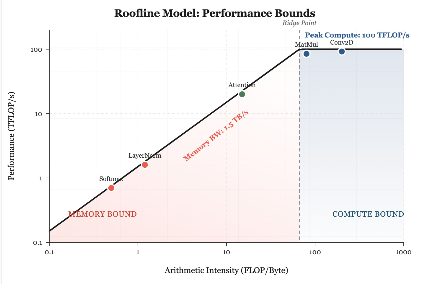
The core idea behind the roofline model is simple. We know every operation carried out on a GPU or TPU must simultaneously use floating-point units and memory channels. Intuitively, the overall speed of that operation is capped by whichever subsystem becomes saturated first! The key value to track here is float-point operations per bytes of memory transferred. This quantity is defined as arithmetic intensity or (FLOP / byte).

A low arithmetic intensity forces the computation to wait on memory bandwidth, effectively making the model and workload “memory bound”. Here, no matter how large and optimized our systolic arrays are for MatMuls, we need to wait on memory transfer as it’s the ‘slower’ between memory transfer and computation.

A high arithmetic intensity, on the other hand, shifts the limitation to the peak FLOP (floating point operation) rate of the physical device. If we plot arithmetic intensity on the x axis and performance (FLOPS or FLOP / seconds, also called throughput) on the y axis, we get the following graph.

High Level: Kernels x Roofline

The position of the kernel relative to these ceilings dictates the performance of the model. This means that once we know whether we are sitting under the memory roof or the compute roof, most “optimization” becomes irrelevant (to an extent, bear with us). The ceiling tells us exactly what kind of improvement is even possible. If the kernel is sitting in the memory bound region, then the hardware is fundamentally starved for data. No amount of code tweaks will magically turn it into a compute heavy kernel. In this case, the only actions that matter are the ones that change how much useful work is done per byte the hardware has to move.

Conversely, if the kernel is against the compute roof, then memory tweaks do nothing, because the limiting resource is the MAC array itself. At that point the only speedups come from reducing the FLOP count or doing something that genuinely increases effective compute throughput. The core point is simple: the roofline gives you the global constraint first, which allows us as computer architects to determine ways to implement hardware (pre-silicon) or software (if post-silicon) fixes to try and eek out all the efficiency we can get. Side note: getting the roofline right and design verification at the earliest stage possible, say RTL as compared to after tape-out is an exponential order of magnitude saved.

Link to Modern ML

So far we’ve only talked about the roofline model in abstract terms. But this matters directly in real ML frameworks because the shape of the kernels your code produces determines where you land on that roofline. Most high-level ML code does not naturally produce big, compute-dense kernels. Our ML workloads today produce tons of small, low–arithmetic-intensity kernels—tiny slices of linear algebra separated by Python overhead, array slicing, broadcasting, reshaping, etc.

On hardware like TPU v1, this is a worst-case scenario. The whole systolic array was designed to run large, regular MatMuls at extremely high utilization. If we feed it a chopped up sequence of micro-operations, we immediately drop into the “memory bound” and “low intensity” region of the roofline, regardless of theoretical peak FLOPs.

In modern ML workloads, a large proportion of the operations that slow down training are not the deep matrix multiplies or convolutions, in fact these often run close to the compute ceiling. Rather, it is the low-intensity operations such as layout conversions, transposes, layer normalization, softmax, and element-wise activations that dominate runtime because they shuttle substantial data through memory for relatively little computation. These operations occupy the far left of the roofline plot, trapped beneath the bandwidth ceiling, and no amount of additional FLOP capacity will accelerate them: hence why a lot of unoptimized ML workloads are memory-bound!

This is also the context in which JAX (the Google compiler framework that traces Python into computation graphs) and XLA (Xcelerated Linear Algebra compiler for computation graphs to fused kernels on device) make sense. When we write high-level JAX code, the Python program is traced into a dataflow graph. JAX or XLA then takes that graph and attempts to fuse as many of those tiny operations as it safely can into a single, larger kernel.

Fusion is the mechanism that raises arithmetic intensity, eliminating memory loads / stores if needed for multiple operations (intuition here is less bytes in the denominator raises arithmetic intensity)! By allowing many low-intensity ops to share memory accesses and remain on-chip, XLA gives the systolic array a more substantial block of work to do, which is more performant. In roofline terms, successful fusion pushes the workload to the right, towards the compute-bound regime, where the accelerator can finally use a meaningful fraction of its peak throughput.

Yet, fusion does not always fix all inefficiencies! Dynamic shapes, incompatible data layouts, indexing patterns, or explicit materializations can force XLA to emit many small kernels. When this happens, the program stays fragmented, and the effective arithmetic intensity collapses. The result is performance pinned under the memory roof. This is the real explanation behind what people casually describe as “slow JAX.” It’s not that JAX has some mysterious overhead or that TPUs secretly dislike a certain tensor shape. The compiler simply cannot fuse the code into a compute-dense kernel, leaving the hardware stuck servicing low-intensity operations. Alternative fixes include tiling, blocking, shifting loops around, and removing atomics (which we will further break down next in this series).

Conclusion

Fragmented compute leads to low arithmetic intensity, which leads directly to memory bound performance. Large fused kernels have high intensity and operate near peak compute on architectures like TPU v1. The roofline model is therefore not only a hardware visualization but also a way of understanding how modern ML frameworks behave and the use of compilers such as XLA.

Works Referenced:

How To Scale Your Model — Roofline Model Overview, jax-ml.github.io/scaling-book/roofline/